July 16th, 2012 | 32 Comments

Sometimes it can be helpful to visualize a third dimension by the color of the line in the plot. For example in Fig. 1 you see a logarithmic sweep going from 0 Hz to 100 Hz. Here the frequency is decoded by the color of the line.

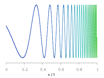
Fig. 1 A logarithmic sweep ranging from 0 Hz to 100 Hz and decoding the frequency with the line color (code to produce this figure, data)

This can be easily achieved by adding a lc palette to the plot command, which uses the values specified in the third row of the data file.

plot 'logarithmic_sweep.txt' u 1:2:3 w l lc palette

The palette can be defined as shown in the Multiple lines with different colors entry. But it can be set in a more easy way, by only setting the start and end color and calculating the colors in between. Therefore, we are picking the two hue values in GIMP (the H entry in Fig. 2 and Fig. 3) for the starting and ending color.

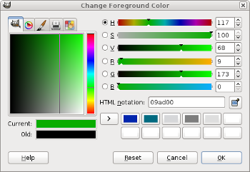
Fig. 2 Picking the HSV value corresponding to the given color of #09ad00.

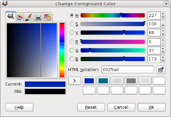
Fig. 3 Picking the HSV value corresponding to the given color of #0025ad.

These colors are then used to specify the palette in HSV mode. The S and V values can also directly be seen in GIMP.

# start value for H
h1 = 117/360.0
# end value for H
h2 = 227/360.0
# creating the palette by specifying H,S,V
set palette model HSV functions (1-gray)*(h2-h1)+h1,1,0.68