July 30th, 2013 | 1 Comment

If you have more than one line or data set in your figure, they has to be named somehow. I’m not a big fan of a legend but prefer to put the names directly to the corresponding curves. That makes it easier for the reader. But as an author of the figure you have to find space to place the labels in the figure, and it could be that you have to rotate the labels to stick them to the lines.

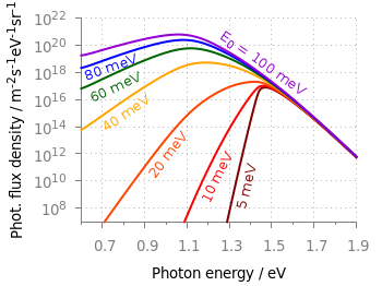
Fig. 1 Photon flux density for different characteristic tail state energies E0 dependent on the photon energy. (code to produce this figure, data)

Figure 1 shows the theoretical curves of photon flux density dependent on the photon energy for different characteristic tail state energies E0. E0 is an indicator for disorder in a crystalline system. To reduce the amount of trail and error for placing the E0 labels, we get the rotation directly from the data by fitting a linear function to the corresponding part of the data.

It is a little bit tricky, because we have a logarithmic y-axis. This can be handled by applying the logarithm to the y data by log($2) and than do the linear fiting.

f(x) = a*x+b
fit [1.30:1.34] [*:*] f(x) 'PL_spectrum_mu_1.0eV_E0_05meV_300K.dat' \
    u 1:(log($2)) via a,b

The first bracket is the range on the x-axis and the second sets the corresponding y range to auto. After we have the value of the slope we convert it to a rotation in degree with the r() function and set our label.

set label 2 '5 meV' at 1.38,4e9 rotate by r(a) center tc ls 1

The conversion to rotation is the most tricky part, because it depends on the range of your axes and the ratio between them. it would be trivial if both axes would go from, for example 1:10 and are equal in length in the figure. Otherwise we have to correct for the ranges and ratio.

# get the relation of x- and y-range
dx = xmax-xmin
dy = log(ymax)-log(ymin)
s1 = dx/dy
# get ratio of axes
s2 = 5/6.7
# helper function for getting the rotation angle of the labels in degree
deg(x) = x/pi*180.0
r(x) = deg(atan(s1*s2*x))