table « Gnuplotting

February 21st, 2014 | 5 Comments

For the measurement of distances T-shaped arrows are often used to highlight the length. In gnuplot there is an easy way to achieve this.

$Diffraction on a slit$

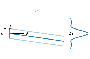
Fig. 1 Diffraction of light for a slit with the length d. (code to produce this figure)

Have a look at Fig. 1 which tries to explain the diffraction phenomenon of a slit with the length d. At a distance a the diffraction pattern is drawn. The different distances, the distance between the first minima of the diffraction pattern, and the wave length are indicated by T-shaped arrows. This kind of arrays can be achieved in gnuplot with the following code.

Theads = 'heads size 0.5,90 front ls 201'
set arrow from -24,-2 to -24, 2       @Theads
set arrow from -22, 2 to -21.44,1.92  @Theads
set arrow from 1.5,-pi to 1.5,pi      @Theads
set arrow from -22,2.5*pi to 0,2.5*pi @Theads

Here, 90 is the relevant entry after size as it describes the opening angle of the arrow head.
In addition, an open circle is drawn to indicate the angle θ. This is achieved by specifying the opening angle for the circle object.

set object circle at -22,0 size 6 arc [-8:0]

Tags: arrow, circle, head, italic, object, table

May 22nd, 2012 | 3 Comments

In one of the last posts we have looked at how to plot equipotential lines. Here we want to plot the equipotential lines of two sources with different charges, like an electron and a positron.

Fig. 1 Equipotential lines of an electron and a positron (code to produce this figure, electron.gnu, positron.gnu)

In addition the sources should be plotted as well, as can be seen in Fig. 1. There the electron is drawn as a red sphere with some lightning effect and the positron as a red sphere. This effect can be achieved with Gnuplot by plotting a bunch of circles with slightly different color and size on top of each other.

set for [n=0:max-1] object n+object_number circle \
    at posx(x,n,max/1.0),posy(y,n,max/1.0) size size(n,max/1.0)
set for [n=0:max-1] object n+object_number \
    fc rgb blue(n,max/1.0) fillstyle solid noborder lw 0

The size and position are determined by the posx,poxy,size functions. The color is chosen according to the blue function for the electron, which is a little tricky and composed of the three color functions r,g,b. These functions generate a color gradient starting from the blue, which is used as the line color for the equipotential lines, into a slight white.

size(x,n) = s*(1-0.8*x/n)
r(x,n) = floor(240.0*x/n)
g(x,n) = floor(144.0*x/n)+96
b(x,n) = floor(67.0*x/n)+173
blue(x,n) = sprintf("#%02X%02X%02X",r(x,n),g(x,n),b(x,n))
posx(X,x,n) = X + 0.03*x/n
posy(Y,x,n) = Y + 0.03*x/n

The code shown so far is put into external functions (electron.gnu, positron.gnu) and can be used in any script to plot equipotential lines, as the one used to generate Fig. 1.

Fig. 2 Equipotential lines of two sources with different charges (code to produce this figure)

The position and size of the source are the parameters of the functions. Fig. 2 shows the result for a negative particle with twice the absolute charge of the positive charged particle.

# positron
x1 = 2; y1 = 1; q1 = 1
# electron
x2 = 1; y2 = 1; q2 = -2
call 'positron.gnu' x1 y1 '0.1'
call 'electron.gnu' x2 y2 '0.2'

Thanks to Gnuplotter for the original idea.

Tags: circle, cntrparam, contour, table

December 18th, 2011 | 12 Comments

In physics equipotential lines describe lines in space which are at the same potential, for example of the electric field.

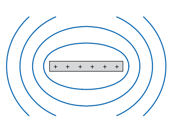
Fig. 1 Equipotential lines of a plate with electric charges (code to produce this figure)

In Fig. 1 equipotential lines for the electric field of six charges equally spaced on a plate are shown. In order to get these lines we need the function of the potential v(x,y) and make a contour plot with splot to a file to save the positions of the lines.

# calculate and save equipotential lines
set view map
unset surface
set contour base
# distance between contour lines according to 1/r
# => equal distance between lines
set cntrparam levels discrete 4,5,6.67,10
set isosam 31,31
set table 'equipotential_lines.txt'
splot v(x,y) w l ls 1
unset table

plot 'equipotential_lines.txt' u 1:2 w l ls 1

The positions of the lines are given by the cntrparam levels which are chosen in a way, to get equally spaced lines in the far field. The set table command stores the contour lines to a file, and finally the last command plots the stored lines.

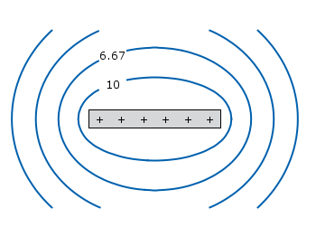
In addition to the equipotential lines the value of the contour is stored as a third column in the equipotential_lines.txt file and can be plotted on the graph, too. This is shown in Fig. 2.

Fig. 2 Equipotential lines of a plate with electric charges with labels (code to produce this figure)

To get the label of the contour we have to choose a x-position which is given by lx0 in the following. The labels(x,y) function sets a string to the value of the third column, if the right x-position is given and we are above the plate. The function f(x,y) checks if we are near the point where a label should be drawn and undefines the contour line around this point. The size of this area is given by eps.

lx0 = 1.14899
eps = 0.15
labels(x,y) = (x==lx0 && y>y0) ? stringcolumn(3) : ""
f(x,y) = (abs(lx0-x)<eps && y>y0) ? 1/0 : y

Tags: cntrparam, contour, label, rectangle, table

May 6th, 2011 | 2 Comments

Fig. 1 A circular loudspeaker array drawn with the object command (code to produce this figure, set_loudspeaker function)

In one of the last entries we have seen how to plot a loudspeaker with Gnuplot.
This time we will have a look at the case of setting more than one loudspeaker to your plot. Furthermore we allow the placement of the loudspeakers after entries in a data file.
Let us assume we have a data file containing the x position, y position and orientation phi of a single loudspeakers per line. Now we have to read the data with Gnuplot and set the objects according to the data. This can be done by a dummy plot, because by applying the plot command, variables can be stored. For the dummy plot we setting the output of the plot command to table and use /dev/null as the place to write the data.

# --- Read loudspeaker placement from data file
set table '/dev/null'
add_loudspeaker(x,y,phi) = sprintf(\
    'call "set_loudspeaker.gnu" "%f" "%f" "%f" "%f";',x,y,phi,0.2)
CMD = ''
plot 'loudspeaker_pos.dat' u 1:(CMD = CMD.add_loudspeaker($1,$2,$3))
eval(CMD)
unset table

The plot command now enables us to add the data from the file to the variable CMD, which is then executed by the eval command. To create the variable, the add_loudspeaker function creates a string with the data for every single line of the data file. The eval(CMD) calls the set_loudspeaker.gnu function once for every single data line, which corresponds to a single loudspeaker. The set_loudspeaker.gnu function itself does the same as we have done in the draw a single loudspeaker entry, but in addition it uses a rotation matrix to change the orientation of the single loudspeakers.

After having set the loudspeakers, we add some activity to three of the loudspeakers and finally get the result in Fig. 1.

# --- Plot loudspeaker activity
set parametric
fx(t,r,phi) = -1.5*cos(phi)+r*cos(t)
fy(t,r,phi) = -1.5*sin(phi)+r*sin(t)
set multiplot
set trange [-pi/6+pi/8:pi/6+pi/8]
plot for [n=1:3] fx(t,n*0.25,pi/8),fy(t,n*0.25,pi/8) w l ls 2
unset object
set trange [-pi/6-pi/8:pi/6-pi/8]
plot for [n=1:3] fx(t,n*0.25,-pi/8),fy(t,n*0.25,-pi/8) w l ls 2
set trange [-pi/6:pi/6]
plot for [n=1:3] fx(t,n*0.25,0),fy(t,n*0.25,0) w l ls 1
unset multiplot

The three waves before the desired loudspeakers are plotted within an iteration that effects the radius by using the for command. The unset object is executed after the first plot in the multiplot environment, because the loudspeakers should only be drawn once.

Tags: call, circle, data, for, iteration, object, parametric, polygon, table

Gnuplotting

Arrow with T-shaped head

Electron and positron

Equipotential lines

Object placement using a data file

Gnuplot Links