filledcurves « Gnuplotting

September 29th, 2014 | 6 Comments

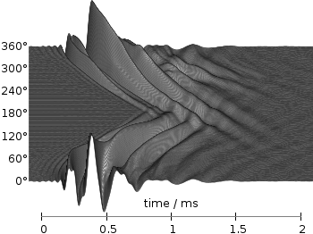
Some time ago I introduced already a waterfall plot, which I named a pseudo-3D-plot. In the meantime, I have been asked several times for a colored version of such a plot. In this post we will revisit the waterfall plot and add some color to it.

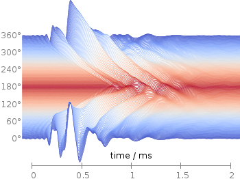
Fig. 1 Waterfall plot of head related impulse responses. (code to produce this figure, color palette, data)

In Fig. 1 the same head related impulse responses we animated already are displayed in a slightly different way. They describe the transmission of sound from a source to a receiver placed in the ear canal dependent on the position of the source. Here, we show the responses for all incident angles of the sound at once. At 0° the source was placed at the same side of the head as the receiver.

The color is added by applying the Moreland color palette, which we discussed earlier. The palette is defined in an extra file and loaded, this enables easy reuse of defined palettes. In the plotting command the palette is enabled with the lc palette command, that tells gnuplot to use the palette as line color depending on the value of the third column, which is given by color(angle).

load 'moreland.pal'
set style fill solid 0.0 border
limit360(x) = x180?360-x:x
amplitude_scaling = 200
plot for [angle=360:0:-2] 'head_related_impulse_responses.txt' \
    u 1:(amplitude_scaling*column(limit360(angle)+1)+angle):(color(angle)) \
    w filledcu y1=-360 lc palette lw 0.5

To achieve the waterfall plot, we start with the largest angle of 360° and loop through all angles until we reach 0°. The column command gives us the corresponding column the data is stored in the data file, amplitude_scaling modifies the amplitude of the single responses, and +angle shifts the data of the single responses along the y-axis to achieve the waterfall.

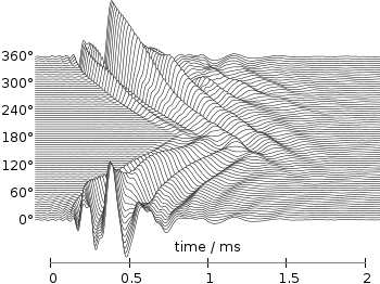
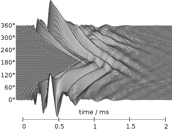
Even though the changing color in the waterfall plot looks nice you should always think if it really adds some additional information to the plot. If not, a single color should be used. In the following the same plot is repeated, but only with black lines and different angle resolutions which also have a big influence on the final appearance of the plot.

Fig. 2 Waterfall plot of head related impulse responses with a resolution of 5°. (code to produce this figure, data)

Fig. 3 Waterfall plot of head related impulse responses with a resolution of 2°. (code to produce this figure, data)

Fig. 4 Waterfall plot of head related impulse responses with a resolution of 1°. (code to produce this figure, data)

Tags: data, fill, filledcurves, for, iteration, palette, style

December 21st, 2013 | 2 Comments

After plotting the world several times we will concentrate on a smaller level this time. Ben Johnson was so kind to convert the part dealing with the USA of the 10m states and provinces data set from natural earth to something useful for gnuplot. The result is stored in the file usa.txt.

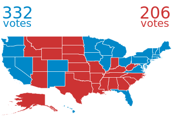
Fig. 1 Election results of single U.S. states. (code to produce this figure, USA data, election data)

Two double lines divide the single states. This allows us to plot a single state with the help of the index command. At the end of this post the corresponding index numbers for every state are listed.
In addition to the state border data we have another file that includes results from an example election and strings with the names of the states. The election result can be 1 or 2 – corresponding to blue and red. With the help of these two data sets we are able to create Fig. 1 and Fig. 2.
For drawing a single state in red or blue we first collect the results for every single state in the string variable ELEC. The stats command is suitable for this, because it parses all the data but doesn’t try to plot any of them. During the parsing of every line the election result stored in the second column will be added at the end of the ELEC variable.

ELEC=''
stats 'election.txt' u 1:(ELEC = ELEC.sprintf('%i',$2))

In a second step we plot the state borders and color the states with the help of the ELECstring. ELEC[1:1] will return the election result for the state with the index 0.

plot for [idx=0:48] 'usa.txt' i idx u 2:1 w filledcurves ls ELEC[idx+1:idx+1],\
                    ''              u 2:1 w l ls 3

Alaska and Hawaii are then added with additional plot commands and the help of multiplot.

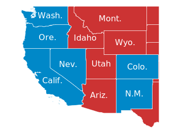
The data file with the election results includes also the names of the single states and a coordinates to place them. This allows us to put them in the map as well, as you can see in Fig. 2.

Fig. 2 Names and election results of single U.S. states. (code to produce this figure, USA data, election data)

The plotting of the state names is easily achieved by the labels plotting style:

plot for [idx=0:48] 'usa.txt' i idx u 2:1 w filledcurves ls ELEC[idx+1:idx+1],\
                    ''              u 2:1 w l ls 3,\
                    'election.txt'  u 6:5:3 w labels tc ls 3

At the end we provide the list with the index numbers and the corresponding states. If you want to plot a subset of states – as in Fig. 2 – you should adjust the xrange and yrange values accordingly.

0  Massachusetts
1  Minnesota
2  Montana
3  North Dakota
4  Idaho
5  Washington
6  Arizona
7  California
8  Colorado
9  Nevada
10 New Mexico
11 Oregon
12 Utah
13 Wyoming
14 Arkansas
15 Iowa
16 Kansas
17 Missouri
18 Nebraska
19 Oklahoma
20 South Dakota
21 Louisiana
22 Texas
23 Connecticut
24 New Hampshire
25 Rhode Island
26 Vermont
27 Alabama
28 Florida
29 Georgia
30 Mississippi
31 South Carolina
32 Illinois
33 Indiana
34 Kentucky
35 North Carolina
36 Ohio
37 Tennessee
38 Virginia
39 Wisconsin
40 West Virginia
41 Delaware
42 District of Columbia
43 Maryland
44 New Jersey
45 New York
46 Pennsylvania
47 Maine
48 Michigan
49 Hawaii
50 Alaska

Tags: data, filledcurves, for, index, labels, multiplot, stats, string

April 3rd, 2013 | 3 Comments

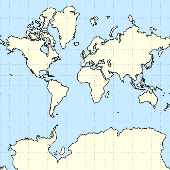
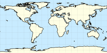
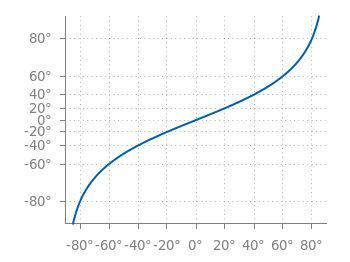
In one of the last posts, we came up with an updated data set representing the world. One way to plot this data set is with a 2D plot, as shown in Fig. 2. But if you compare the output with the one you see for example at Google Maps you will noticed a difference. That is due to the fact that Google uses the Mercator projection of the data. This projection preserves the angles around any point on the map, what is useful if you have a close look at some streets. The disadvantage of the Mercator projection is the inaccuracy of the sizes of the countries near to the poles. For example the size of Greenland is completely overemphasized as you can see in Fig. 1.

Fig. 1 Mercator projection of the world (code to produce this figure, data)

In order to achieve the Mercator projection, we apply the following function.

set angles degrees
mercator(latitude) = log( tan(180/4.0 + latitude/2.0) )
set yrange [-3.1:3.1]
plot 'world_110m.txt' u 1:(mercator($2)) w filledcu ls 2

Fig. 2 Equirectangular projection of the world (code to produce this figure, data)

By just plotting the data as we have done for Fig. 2, we have the Equirectangular projection with constant spacing between the latitudes and meridians. The blue background color in the first two figures can be achieved directly with a terminal setting.

set terminal pngcairo size background '#c8ebff'

Fig. 3 Mapping of the Mercator projection (code to produce this figure)

In Fig. 3 the Mercator projection function is shown as an input-output-function of the latitude values. The placing of the latitude values on the y-axis can be easily done with a loop.

set ytics 0
do for [angle=-80:80:20] {
    set ytics add (sprintf('%.0f',angle) mercator(angle))
}

Tags: background, data, do, filledcurves

February 6th, 2013 | 8 Comments

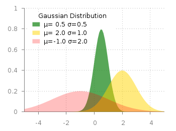
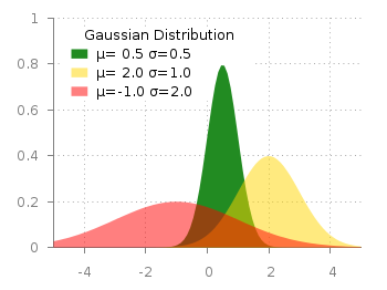
Maybe you all know the nice example of gnuplots transparent fill style. I have replotted it slightly modified in Fig. 1.

Fig. 1 Filledcurves with transparency settings as on the gnuplot demo site (code to reproduce this figure)

The interesting part in the code looks like this.

set style fill transparent solid 0.5 noborder
plot d1(x) fs solid 1.0 lc rgb "forest-green" title 'µ= 0.5 σ=0.5', \
     d2(x) lc rgb "gold" title 'µ= 2.0 σ=1.0', \
     d3(x) lc rgb "red" title 'µ=-1.0 σ=2.0'

The set style command sets the fill style to 50% transparency, which is overwritten by the explicit fs option to the first plotting command in order to plot the green curve without transparency.

Fig. 2 Filledcurves with different transparency settings (code to reproduce this figure)

Now the question is how to plot filled curves with different transparency settings? The simple answer is, by just using this explicit fs plot argument. The result is shown in Fig.2 and can be reached with the following code. Now we apply a transparency of 75%, 50%, and 25% going from the green to the red curve.

set style fill noborder
plot d1(x) fs transparent solid 0.75 lc rgb "forest-green" \
        title 'µ= 0.5σ=0.5', \
     d2(x) fs transparent solid 0.50 lc rgb "gold" \
        title 'µ= 2.0 σ=1.0', \
     d3(x) fs transparent solid 0.25 lc rgb "red" \
        title 'µ=-1.0 σ=2.0'

Tags: fill, filledcurves, transparent

October 10th, 2011 | No Comments

In the last entry we have seen how to use a color map to represent matrix data. Another way to visualize such kind of data is to code their values not as color, but as height information using so called pseudo 3D plots.

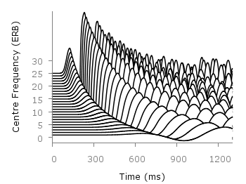
Fig. 1 Pseudo 3D plot of basilar membrane activity (code to produce this figure, data)

Suppose we have some data like spectra with different parameters, slightly shifted and plotted into the same figure, or different oscillations over time as shown in Fig. 1. There, the movement of the basilar membrane to an input stimuli dependent on the center frequency in ERB is plotted over time. The movement on the basilar membrane is dependent on the frequency of the incoming stimulus, with different frequencies acting on different places along the membrane. In order to plot this kind of data the for command of Gnuplot can be used to iterate through the data. The pseudo 3D effect is realized by shifting the data in every iteration one ERB by the +ii part and the usage of filledcurves to overwrite not visible parts of the plot with white color.

set style fill solid 1.0 border rgb 'black'
plot for [ii=25:1:-1] 'bmm.txt' u (f(column(ii))+ii) \
    w filledcu y1=-2 ls 1

The amplitude of the data was originally stored in order to fit in a plot given in Hz. Hence, we have to convert the data into ERB. This is done by the function f. As arguments to the function the values of each column are given in the iteration. Therefore, the column number is indexed by the column function.

Tags: data, filledcurves, for, iteration

June 24th, 2011 | No Comments

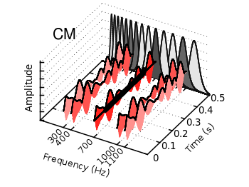
The filledcurves style is only available for 2d plots. But it can be used with some limitations with splot in 3d plots as well. In this entry we want to visualize an effect known from psychoacoustics, called comodulation masking release. The effect describes the possibility of our hearing system to perceive a masked tone (in this case at 700 Hz) easier in the presence of so called comodulated maskers present in other auditory filters. Comodulation describes the fact, that all maskers have the same envelope, as can be seen in Fig. 1.

Fig. 1 Visualization of the comodulation masking release using splot and filledcurves (code to produce this figure, gfb_loop.gnu, gfb.dat, sig.dat, noise.dat)

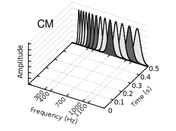
First we start with the gammatone filters. The values for them are stored in the gfb.dat file as one column per filter. In order to apply different colors to different filters the style function sty(x) is defined. The data(x) function is defined to be able to plot the filters in a particular order. This will result in the nice effect of overlapping filters shown in Fig. 2.

sty(x) = x<7 ? 1 : x<10 ? 2 : x<12 ? 1 : x==12 ? 3 : x<15 ? 1 : \
    x==15 ? 2 : 1
data(x) = x<12 ? x : 29-x

The filter bank itself is plotted by the gfb_loop.gnu function. There the data are plotted first as filledcurves and then as a line. This two step mechanism has to be used, because the filledcurves style is not able to draw an extra line in 3d. Hence it has to be done in the extra gfb_loop.gnu function, because the simple for iteration only works for a single plot and is not able to plot the line around the filters.

# gfb_loop.gnu
splot 'gfb.dat' u 2:1:(column(data(i))) w filledcurves \
    ls sty(data(i)), \
      ''        u 2:1:(column(data(i))) ls 4
i = i+1
if (i<maxi) reread

Fig. 2 Plotting gammatone filters with an extra loop file (code to produce this figure, gfb_loop.gnu, gfb.dat)

Thereafter the modulated noise and its envelope and the signal are plotted in different parts of the graph by explicitly giving the x position.
The result is shown in Fig. 1.

splot 'noise.dat' u  (300):1:2 ls 11, \
      ''          u  (300):1:3 ls 14, \
      ''          u  (400):1:2 ls 12, \
      ''          u  (400):1:3 ls 14, \
      ''          u  (700):1:2 ls 13, \
      ''          u  (700):1:3 ls 14, \
      ''          u (1000):1:2 ls 12, \
      ''          u (1000):1:3 ls 14, \
      ''          u (1100):1:2 ls 11, \
      ''          u (1100):1:3 ls 14
splot 'sig.dat'   u  (700):1:2 ls 14

Tags: call, filledcurves, iteration, reread, splot

Gnuplotting

Waterfall plots with changing color

U.S. states and election results

Mercator projection

Filledcurves with different transparency

Creating pseudo 3D plots

Filledcurves with splot

Gnuplot Links