Gnuplotting

Create scientific plots using gnuplot

June 23rd, 2014 | 8 Comments

Occasionally it is a good idea to create a zoom of some part of your main plot, especially if you have a small part of your plot where the data is hiding each other.
Including a zoom with multiplot

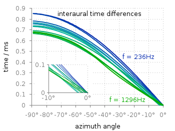
Fig. 1 Including a zoom into your figure to emphasize some data. (code to produce this figure, data)

In Fig. 1 the interaural time difference between a sound signal reaching the two ears of a listener is plotted with different colors for different frequencies. The data is very dense around 0°, so we include a zoom into this region in the same figure at a free place.

This can be done via multiplot and the plotting of the same data in a smaller figure.

set origin 0.12,0.17
set size 0.45,0.4
set xrange [-10:0]
set yrange [0:0.1]
plot for [n=2:13] 'itd.txt' u 1:(column(n)*1000) w lines ls n

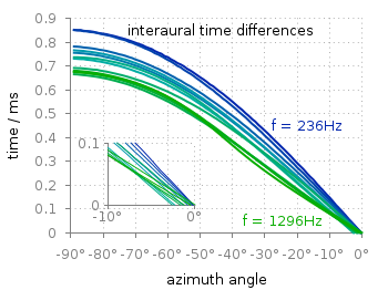
The tricky part is that we have a grid in our main figure and if we do nothing the grid will also be visible in the zoomed in version as shown in Fig. 2.
Including a zoom with multiplot without grid correction

Fig. 2 Including a zoom into your figure, without correcting the grid. (code to produce this figure, data)

To avoid this we have to hide the grid in the background of the zoomed graph. This is done with the trick of placing an empty white rectangle at the place the zoom plot should appear in the figure.

set object 1 rect from -88,0.03 to -49,0.41
set object 1 rect fc rgb 'white' fillstyle solid 0.0 noborder

This will then finally lead to the desired result presented in Fig. 1.
December 18th, 2011 | 12 Comments

In physics equipotential lines describe lines in space which are at the same potential, for example of the electric field.

Equipotential lines

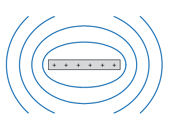
Fig. 1 Equipotential lines of a plate with electric charges (code to produce this figure)

In Fig. 1 equipotential lines for the electric field of six charges equally spaced on a plate are shown. In order to get these lines we need the function of the potential v(x,y) and make a contour plot with splot to a file to save the positions of the lines.

# calculate and save equipotential lines
set view map
unset surface
set contour base
# distance between contour lines according to 1/r
# => equal distance between lines
set cntrparam levels discrete 4,5,6.67,10
set isosam 31,31
set table 'equipotential_lines.txt'
splot v(x,y) w l ls 1
unset table

plot 'equipotential_lines.txt' u 1:2 w l ls 1

The positions of the lines are given by the cntrparam levels which are chosen in a way, to get equally spaced lines in the far field. The set table command stores the contour lines to a file, and finally the last command plots the stored lines.

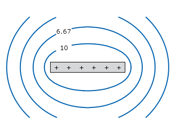
In addition to the equipotential lines the value of the contour is stored as a third column in the equipotential_lines.txt file and can be plotted on the graph, too. This is shown in Fig. 2.

Equipotential lines with labels

Fig. 2 Equipotential lines of a plate with electric charges with labels (code to produce this figure)

To get the label of the contour we have to choose a x-position which is given by lx0 in the following. The labels(x,y) function sets a string to the value of the third column, if the right x-position is given and we are above the plate. The function f(x,y) checks if we are near the point where a label should be drawn and undefines the contour line around this point. The size of this area is given by eps.

lx0 = 1.14899
eps = 0.15
labels(x,y) = (x==lx0 && y>y0) ? stringcolumn(3) : ""
f(x,y) = (abs(lx0-x)<eps && y>y0) ? 1/0 : y