Gnuplotting

Create scientific plots using gnuplot

December 1st, 2012 | 7 Comments

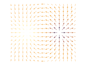
In an earlier entry we created a vector field from measured data. Now we will visualize functions with the vector plotting style. As functions we have two 1/r potentials which define the amplitude of the vectors, as can be seen in Fig. 1. It is often better to indicate the amplitude by a color instead of by the length of the single vectors, especially if there are big changes. For the exact functions have a look into the corresponding file.
Vector field showing two sources

Fig. 1 Vector field of two sources with the opposite charge. The color indicates the amplitude. (code to produce this figure)

By analogy to the data vector field we have again a dx, and dy function for the length of the vectors.

dx(x,y) = scaling*ex(x,y)/enorm(x,y)
dy(x,y) = scaling*ey(x,y)/enorm(x,y)

Now we need a trick, because we have to fill the u 1:2:3:4 for the vector style with our function data. The four columns are then x,y,dx,dy of the vectors, where dx, dy are the lengths of the vector in x and y direction. Here the special filename ++ is a big help. It gives us x and y points as a first and second column, which we could address by $1 and $2. The number of points for the two axes are handled by the samples and isosamples command.

set samples 17    # x-axis
set isosamples 15 # y-axis
plot '++' u ($1-dx($1,$2)/2.0):($2-dy($1,$2)/2.0):\
    (dx($1,$2)):(dy($1,$2)):(v($1,$2)) \
    with vectors head size 0.08,20,60 filled lc palette

To place the vector at the center of the single x, y points, we move the starting point of the vectors to x-dx/2, y-dy/2.
July 8th, 2011 | 1 Comment

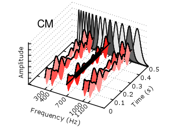
The last entry has plotted all its data from data files, even the signal at 700Hz. In this entry we will see how to plot the signal as a function using the special-filenames property of Gnuplot.

CMR

Fig. 1 Visualization of the comodulation masking release using splot and special-filenames (code to produce this figure, gfb_loop.gnu, gfb.dat, noise.dat)

In Fig. 1 the end result is seen. What we have done is to replace the last splot command from the cmr.gnu file with the following code.

set samples 500
# Define the sinusoid signal to be plotted
sig(y) = y>0.1 && y<0.4 ? 0.45*sin(2*pi*100*y)+2 : 2
# The desired range is 0:0.5, but the samples were created for the
# x-axis, which has a range of 0:1400, therefore we calculate an
# factor to do the plot
fact = 1400/0.5
splot '+' u (700):($1/fact):(sig($1/fact)) w l ls 14

We define the function sig(y) which is a 100Hz sinusoid centered at 2 for values of y between 0.1 and 0.4 and constant 2 else. In order to place this two dimensional function in our 3D plot we use the special-filenames property from Gnuplot, in this case the '+' variant. This tells Gnuplot to use the xrange, apply a sampling of it and return it as first column for the plot command. But for our plot we need the y-axis and not the x-axis, because the x values should be constant at 700 and are therefore given by (700) at the splot command. The values of the first column, given by $1 are scaled by fact in order to match the two axis and are then directly used as y values and given to the sig(y) function for the z values.

August 13th, 2010 | 7 Comments

In Gnuplot it is easy to define a continuous and differentiable function such as f(x) = x, but what to do if we need a function that fulfill non of these conditions?
For example let us consider a step function. Typically a step function is given by

           / 1   if x > a
step(x) = -|
           \ 0   else

In Gnuplot this can be achieved by using the ternary operator:

step(x) = x>a ? 1 : 0

Which is a simple if-else statement and means step(x)=1 if x>a else step(x)=0.

If we plot this function we get Fig. 1.

step function

Fig. 1 Continuous plot of the step function (code to produce this figure)

As you can see this will result in a continuous plot. If we want a discontinuity in the plot, we have to create two separate functions that are only piecewise defined. This can be achieved by using 1/0 that will result in a undefined value.

f(x) = x<a  ? 1 : 1/0
g(x) = x>=a ? 1 : 1/0 

Plotting both functions will result in Fig. 2.

step function

Fig. 2 Discontinuous plot of the step function (code to produce this figure)

The ternary operator can also be used in an iterative way. For example if we want to define a rectangular function that is given by

           / 0     if abs(x) > 0.5
rect(x) = -| 0.5   if abs(x) = 0.5
           \ 1     if abs(x) < 0.5

we can use the following statement in Gnuplot to define it:

rect(x) = abs(x)>0.5 ? 0 : abs(x)<0.5 ? 1 : 0.5

In Fig. 3 you can see a plot of this function. To produce the sharp edges of the rectangular function we use a higher number of sampling points (also in Fig. 1 for the step function). In order to plot a function Gnuplot calculates 100 points of the given function and draw a line through them. This can be set to another value with the set samples <value> command.

rectangular function

Fig. 3 Plot of the above defined rect(x) function (code to produce this figure)